


Overview
Real-world data distributions evolve over time, inducing temporal distribution shift that can substantially degrade the reliability of deployed machine learning systems.
We present a systematic empirical comparison of temporal robustness across three heterogeneous, time-indexed domains encompassing image classification, multi-label text classification, and text regression tasks. Using a unified evaluation framework based on temporal drift matrices, we train models on cumulative historical data and evaluate their performance on both earlier and later time periods.
Collectively, the results characterize how temporal drift degrades performance as the train-test gap widens across domains, drift scenarios, and model families, offering practical guidance for selecting architectures for dynamic systems; across all settings, inductive biases aligned with domain structure yield markedly greater temporal robustness.
Paper Contributions
(I) Cross-Domain Temporal Study
Systematic evaluation of temporal robustness across heterogeneous domains and task types, rather than a single benchmark.
(II) Unified Temporal Evaluation Framework
Model-agnostic protocol based on cumulative historical training and temporal drift matrices, yielding comparable robustness measurements across datasets, tasks, and metrics.
(III) Architectural Inductive Bias Analysis
Large-scale comparison of diverse neural architectures to quantify how differing inductive biases shape robustness under temporal shift.
Types of Temporal Drift
Following Gama et al. (2014), temporal distribution shift manifests along three axes:
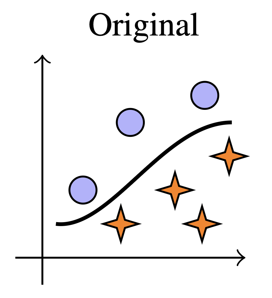
Original Distribution
Circles and stars indicate the two label classes and the curve represents the decision boundary.
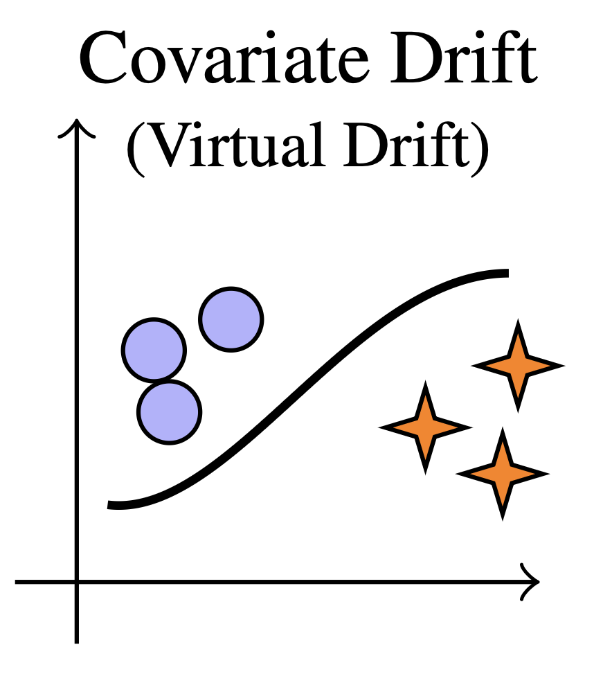
Covariate Shift
P(X) changes, P(Y|X) fixed
Input distribution evolves (e.g., hairstyles, image quality) while the labeling function remains stable.
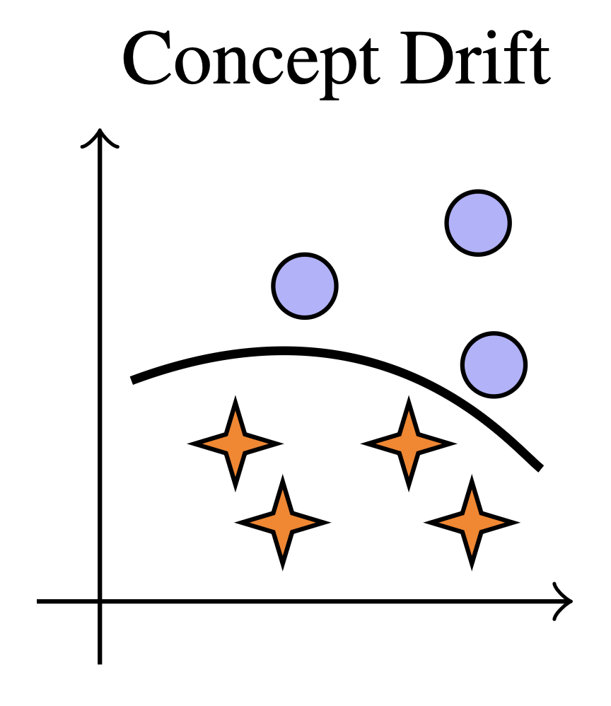
Concept Drift
P(Y|X) changes
The relationship between inputs and labels shifts—same text may indicate different categories over time.
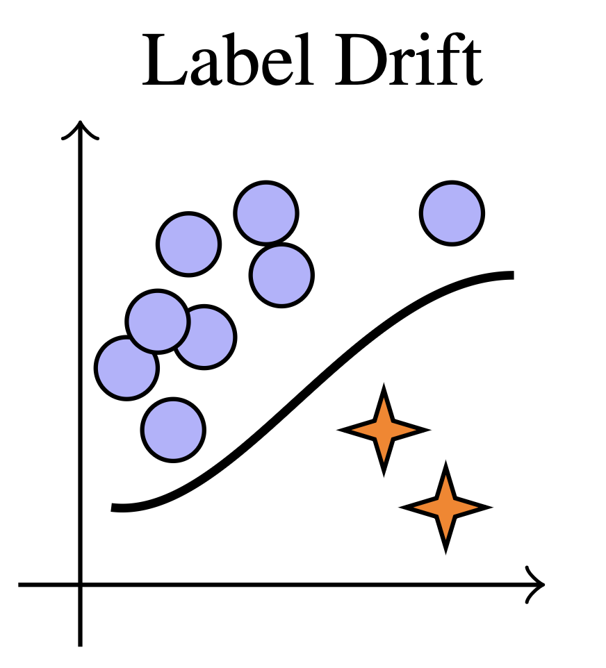
Label Shift
P(Y) changes
Class prevalence evolves as research topics or product categories rise and fall in popularity.
Datasets
1905–2013
Yearbook
Standardized portraits of U.S. high-school seniors with binary sex labels. Pronounced covariate and concept drift from evolving hairstyles, clothing, and photographic artefacts makes it a canonical long-range benchmark.
1986–2025
arXiv
2.87M article titles annotated with 176 subject categories (restricted to the five most frequent). Topic prevalence and terminology change over decades, inducing label and vocabulary drift in this multi-label setting. We use a sample of 360,265 articles across the top 5 categories.
1996–2023
Amazon Reviews
571M reviews spanning 33 categories; we uniformly sample 100K reviews from seven categories to capture covariate and concept drift in consumer language. Strong rating skew motivates balanced error metrics. We only use a sample of 100,000 reviews across 7 categories.
Models
Image Models (Yearbook)
Two to five fully connected layers (199K-1.1M parameters) trained from scratch on flattened 32x32 pixels. Provide a low-capacity reference with no spatial inductive bias.
Wild-Time baseline plus VGG-, AlexNet-, deep, and wide variants (29K-2.9M parameters) explore locality, depth, and receptive field width under convolutional inductive biases.
Residual networks with two or three stages (660K-2.8M parameters) trained from scratch; skip connections stabilize deeper hierarchies for small portraits.
DINOv2-S, DINOv3-S, CLIP-B/32, ConvNeXt-S, EVA02-B, and SigLIP-B provide frozen feature extractors (770 - 3k trainable classifier head parameters); we train only linear heads to isolate the benefit of large-scale pretraining.
Text Models (arXiv, Amazon)
Frozen RoBERTa embeddings are mean-pooled and fed into a two-layer MLP (39M trainable parameters) with varying dropout (baseline, low, high); discards word order entirely.
Convolutional text classifiers with kernels spanning 2-5 tokens over learnable embeddings (6.6M-39M trainable parameters), capturing local n-gram statistics without long-range context.
Bidirectional GRU and LSTM models (6.6M-15.5M trainable parameters) with learned embeddings process sequences token-by-token; the largest adds attention pooling over hidden states.
Lightweight Transformer encoders with 2, 3, or 6 layers (6.9M trainable parameters) use learned positional embeddings and mean pooling to capture long-range dependencies.
Adam optimizer with cumulative temporal training; weighted binary cross-entropy for arXiv and rating-balanced mean squared error for Amazon.
Temporal Drift Matrices
We adopt a cumulative-historical protocol: train on all data up to period \(k\), then evaluate on every period.
Each entry \(M_{ij}\) measures performance of model \(f_i\) (trained through period \(i\)) when evaluated on period \(j\). This reveals both forward generalization (\(j > i\)) and backward consistency (\(j < i\)), where backward evaluation uses only held-out validation and test splits to prevent data leakage.
Matrix Interpretation
For evaluation periods already included in training (\(j \le i\)), we use only held-out validation and test splits to avoid leakage; for \(j > i\), every available sample becomes out-of-distribution test data so forward estimates remain high-signal.
Cumulative models \(f_i\) are trained with Adam on all data up to slice \(i\). Yearbook minimizes cross-entropy, arXiv uses class-weighted binary cross-entropy per label, and Amazon minimizes rating-weighted mean squared error to counter strong label imbalance.
Binary accuracy populates Yearbook drift matrices, macro-AUC (uniformly averaged over five categories) summarizes arXiv, and balanced MSE averages per-rating errors so rare 1- and 2-star reviews remain visible.
Example of average accuracy matrix computed on a group of Yearbook models.
Image Classification (Yearbook)
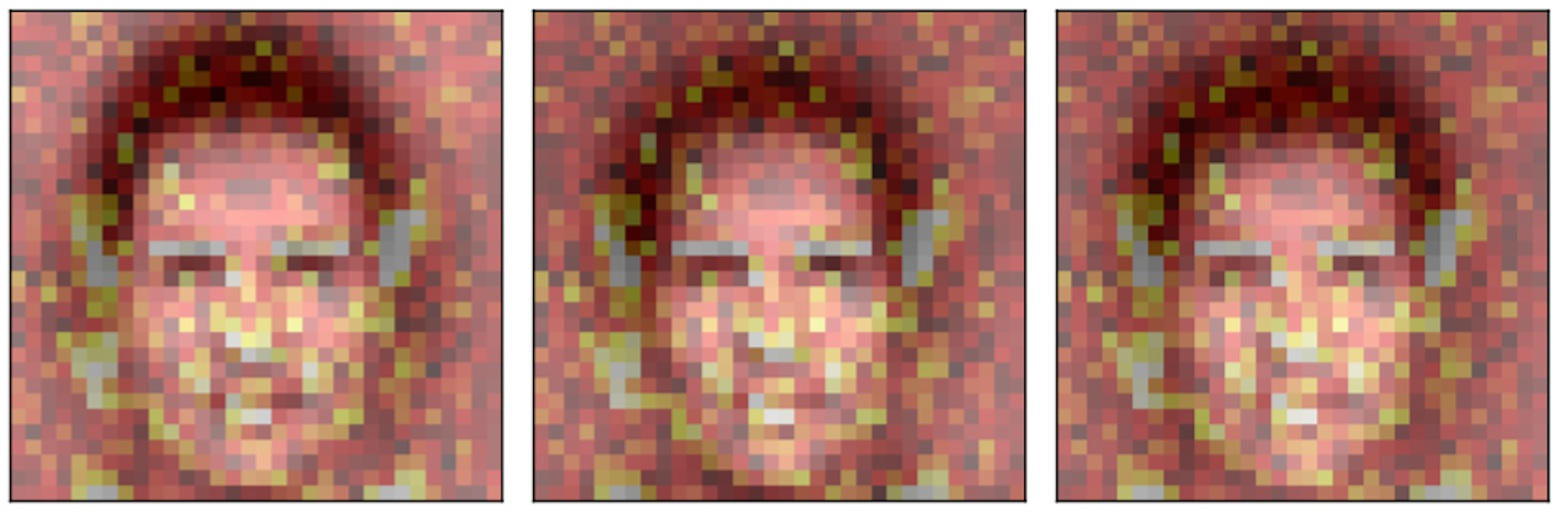
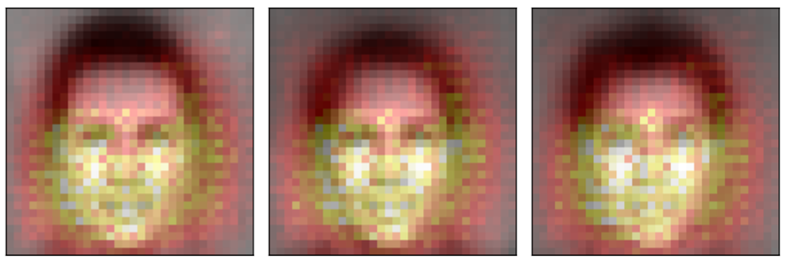
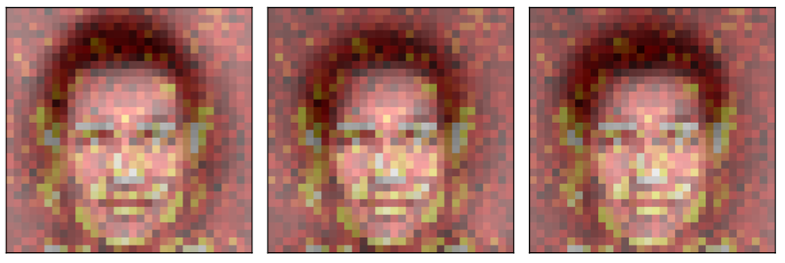
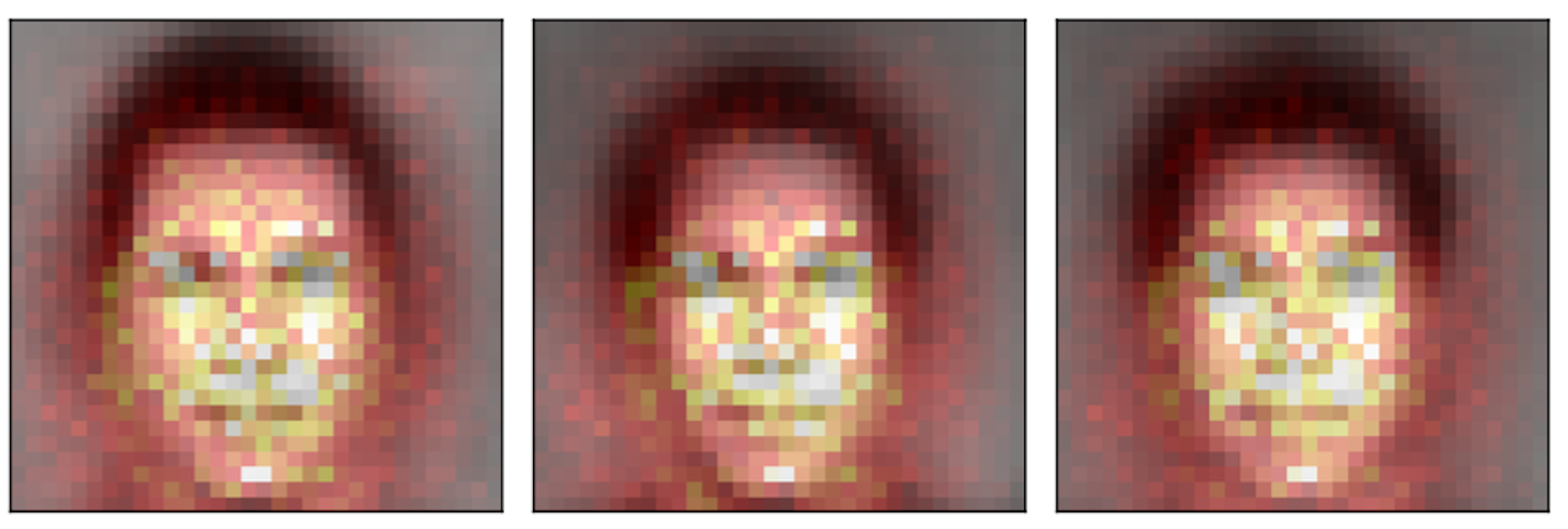
Average faces from the Yearbook dataset across decades.
Performance
Most robust scratch-trained model. Diagonal accuracy >93%, smallest forward decay. Hierarchical features remain stable across the mid-century fashion transition.
High diagonal (mid-90s), but 10-20pt drop on future decades. Performance collapses sharply post-1970s as hairstyles and accessories change.
Largest degradation—over 15pt loss on future data. Relies on global pixel statistics: hair silhouette, background intensity.
Frozen backbones (self-supervised and vision-language) yield lower peak accuracy yet single-digit forward decay, trading specialization for smoother temporal performance.
Saliency Analysis
We compute gradient-based saliency maps to visualize which image regions each architecture attends to, explaining observed robustness differences.
Broad, noisy attribution over hair, clothing, and background—features that change significantly across decades.
Concentrated on inner facial regions (eyes, nose, mouth), stable across decades. Down-weights peripheral regions.
Architectures that focus on temporally stable semantic features (facial structure) exhibit higher cross-temporal robustness.
(a) ResNet-Small
(b) MLP-Small
(c) CNN-Baseline
Text Classification & Regression
Across arXiv (macro-AUC) and Amazon Reviews (balanced MSE), early training slices degrade as the evaluation window moves forward, less dramatically than Yearbook yet enough to expose architectural differences.
arXiv (Multi-label, Macro-AUC)
Order-agnostic pooling exhibits the steepest forward decay: models trained on 2000-era data lose >0.05 macro-AUC when evaluated post-2015 because new terminology shifts the embedding statistics.
Local convolutional filters over embeddings remain surprisingly brittle. Despite competitive diagonal scores, drift matrices show sharp drops for models trained before 2010.
Bidirectional GRU/LSTM variants achieve the flattest drift matrices: sequential inductive biases capture syntactic structure that changes slowly, yielding small deviations even far from the training slice.
Lightweight Transformers match RNN diagonal performance but show moderate forward decay, landing between recurrent robustness and the drift sensitivity of TextCNN.
Figure 3: Drift Matrix — arXiv (Transformer, Macro-AUC)
Amazon Reviews (Regression, Balanced MSE)
Bag-of-embeddings baselines underperform both diagonally and forward-in-time. Ignoring word order makes them sensitive to shifts in review phrasing and platform-specific jargon.
Convolutional models show high variance across configurations and suffer pronounced future degradation despite strong local feature extraction.
GRU, LSTM, and LSTM-Attn variants deliver the lowest balanced MSE overall and the most stable forward trajectories—temporal drift barely nudges their error maps.
Transformer encoders benefit from parallel self-attention yet still exhibit more drift than recurrent counterparts, underscoring the utility of explicit sequential inductive bias.
Figure 4: Drift Matrix — Amazon (Transformer, Balanced MSE)
Central Observation
Architectures whose inductive biases match domain structure (spatial locality for faces, sequential modeling for text, broad coverage from pretraining) retain accuracy far longer under temporal distribution shift.
Summary
In-distribution ≠ Temporal Robustness
High held-out accuracy does not predict cross-temporal generalization. Evaluation must explicitly measure forward drift.
Inductive Biases Determine Robustness
Architectures whose biases match domain structure—spatial hierarchy for images, sequential modeling for text—degrade more gracefully.
ResNets Most Robust for Images
Among scratch-trained models, ResNets show smallest forward decay; MLPs are most drift-sensitive due to reliance on global statistics.
Pretraining Smooths Degradation
Large-scale pretraining yields lower peak accuracy but flatter decay curves—trading specialization for temporal stability.